
QTL mapping has evolved significantly over the last 30 years. Each method—from simple single-marker tests to multi-QTL models—represents a step forward in power, resolution, and biological insight.
Here is a practical overview for everyone who want to understand how these methods work and what each can (and cannot) do.
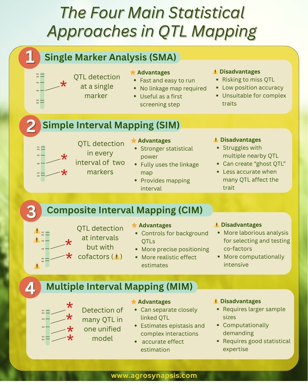
1️⃣ Single Marker Analysis (SMA)
The analysis for QTL detection is done at a single marker each time.
The idea is simple: if a marker is close to a QTL, genotypic classes will differ in their trait means. Tests such as ANOVA, regression, or t-tests are used.
⭐ Advantages
Fast and easy to run
Does not require a linkage map
Useful as a first screening step
⚠️ Disadvantages
High chance of missing QTL
Very low positional accuracy
Cannot detect QTL between markers
Unsuitable for complex traits
Precision: very low
2️⃣ Simple Interval Mapping (SIM)
SIM evaluates the likelihood of a QTL in very interval between two markers.
Using the linkage map and recombination frequencies, it computes a LOD score across the genome. A QTL is inferred where the LOD exceeds the threshold.
⭐ Advantages
Stronger statistical power than SMA
Detects QTL between markers
Fully uses the linkage map
Precision: moderate — improved localization and stronger signals
⚠️ Disadvantages
Struggles with multiple nearby QTL
Can create “ghost QTL” if background effects are not controlled
Less accurate when many QTL affect the trait
3️⃣ Composite Interval Mapping (CIM)
CIM tests a genome interval for a QTL while controlling for other marker effects. First, significant markers (cofactors) are selected via stepwise regression. Then, for each interval, cofactors outside the test window are included in the model to block background genetic variation.
⭐ Advantages
Higher detection power than SIM
Controls for background QTL
Produces sharper LOD peaks
More realistic effect estimates
Precision: high — good resolution, fewer false positives
⚠️ Disadvantages
Results depend on cofactor selection
More computationally intensive
Can still miss QTL if cofactors overlap or window sizes are poorly chosen
4️⃣ Multiple Interval Mapping (MIM)
MIM is a multiple-QTL method because it simultaneously estimates the number, position, and effects of several QTL in one unified model.
⭐ Advantages
Most biologically realistic QTL model
Can separate closely linked QTL
Estimates epistasis and complex interactions
Most accurate effect estimation
Precision: very high — best localization and modeling capacity
⚠️ Disadvantages
Requires larger sample sizes
Computationally demanding
Requires good statistical expertise
👉 If you’d like to be informed about the upcoming workshops organized by AgroSynapsis, and receive early access and discounts, 𝗳𝗶𝗹𝗹 𝗼𝘂𝘁 𝗼𝘂𝗿 𝘀𝗵𝗼𝗿𝘁 𝘁𝗿𝗮𝗶𝗻𝗶𝗻𝗴 𝗶𝗻𝘁𝗲𝗿𝗲𝘀𝘁 𝗳𝗼𝗿𝗺 here: